In this article, we will explain the past and present life of deep learning from the perspective of code. The article explains the different stages according to the six pieces of code, and uploads related code examples. If you are new to FloydHub, after installing the CLI in the sample project folder on your local machine, you can start the project on FloydHub with the following command:

Next, let's follow the original author to read the six historically significant code, least squares method.
The least squares method was originally proposed by the French mathematician Adrien-Marie Legendre, who was known for his participation in the development of standard meters. Legendre is obsessed with predicting the position of the comet, based on the positions where the comet has appeared, and the indomitable calculation of the orbit of the comet. After experiencing numerous tests, he finally came up with a way to balance the calculation error, followed by its 1805. This idea was published in the book "The New Method of Computation of the Comet Orbit", known as the least squares method.
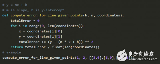
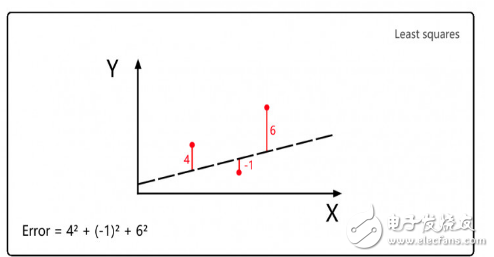
Legendre uses the least squares method to calculate the orbit of the comet. The first is to guess the position of the comet in the future, and then calculate the square error of the guess. Finally, the corrected guess is used to reduce the sum of the squared errors. This is the linear regression idea. source.
Execute the code above on the Jupyter notebook. m is the coefficient, b is the prediction constant, and XY coordinates represent the position of the comet, so the goal of the function is to find a combination of a particular m and b so that the error is as small as possible.
This is also the core idea of ​​deep learning: given input and expected output, looking for the correlation between the two.
Gradient descent
Legendre's method is to find the specific combination of m and b in the error function to determine the minimum error, but this method requires manual adjustment of parameters. This manual adjustment to reduce the error rate is very time consuming. A century later, the Dutch Nobel laureate Peter Debye improved the method of Legendre.
Suppose that Legendre needs to correct a parameter X, and the Y axis represents the error of different X values. Legendre hopes to find such an X, so that the error Y is minimal. As shown in the figure below, we can see that when X=1.1, the value of error Y is the smallest.
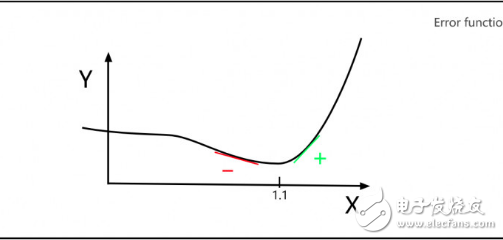
As shown above, Derby notes that the slope to the left of the minimum is a negative number and the slope to the right of the minimum is a positive number. Therefore, if you know the slope of the X value at any point, you can determine whether the minimum Y value is to the left or the right of this point, so next you will try to choose the X value in the direction close to the minimum value.
This introduces the concept of gradient descent, and almost all deep learning models apply gradient descent.
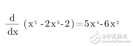
Assume the error function Error = X5 - 2X3 - 2
Derivate to calculate the slope:
If you need to supplement the knowledge of the derivative, you can learn the video of Khan Academy.
The python code in the following figure explains the mathematical method of Derby:
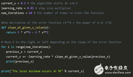
The most noteworthy code in the above figure is the learning rate, learning_rate, which slowly approaches the minimum by moving in the opposite direction of the slope. As you get closer to the minimum, the slope becomes smaller and smaller, slowly approaching zero, which is the minimum.
Num_iteraTIons represents the number of iterations estimated before the minimum is found.
Running the above code, the reader can adjust the gradient to familiarize himself with the gradient drop.
Linear regression
The linear regression algorithm combines the least squares method with gradient descent. In the 1950s and 1960s, a group of economists realized the early ideas of linear regression on early computers. They use perforated paper to bring programming, which is a very early computer programming method that scans the computer into a computer by placing a series of regular holes on the tape. Economists spent several days punching, and it took more than 24 hours to run a linear regression on an early computer.
The figure below is a linear regression of Python implementation.
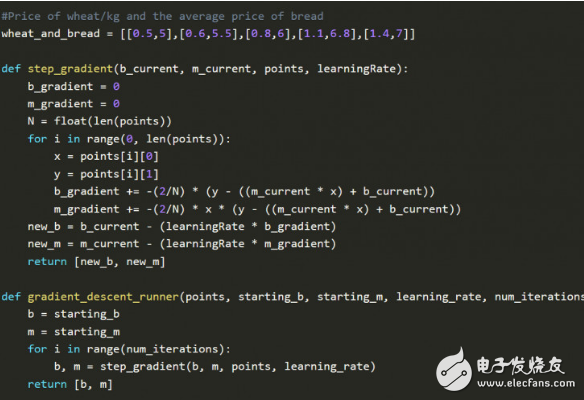
Gradient descent and linear regression are not new algorithms, but the combination of the two is still amazing. Try this linear regression simulator to familiarize yourself with linear regression.
Perceptron
The perceptron was first proposed by Frank Rosenblatt, a psychologist at Cornell Aviation Labs. In addition to studying brain learning and hobbies, Rosenblatt can analyze bat research and migration during the day. The ability to go to the top of the house at night to build an observatory to study outer space life. In 1958, Rosenblatt simulated neuron invented the perceptron and boarded the New York Times headline with a New Navy Device Learns By Doing.
Rosenblatt’s machine quickly attracted the attention of the public, giving the machine 50 sets of images (each consisting of a logo to the left and a logo to the right) without pre-programmed commands. In this case, the machine can recognize the direction of the picture.
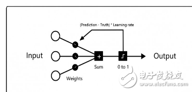
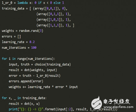
Each training process starts with the input neurons on the left, assigns random weights to each input neuron, and then calculates the sum of all weighted inputs. If the sum is negative, the marker prediction result is 0, otherwise the marker prediction The result is 1.
If the prediction is correct, there is no need to modify the weight; if the prediction is wrong, multiply the learning rate (learning_rate) by the error to adjust the weight accordingly.
Let's take a look at how the perceptron solves traditional or logical (OR).
Python implementation perceptron:
After people's excitement about the perceptron, Marvin Minsky and Seymour Papert broke the cult of this idea. At the time, Minsky and Paptt both worked at MIT's AI lab. They wrote a book to prove that the perceptron can only solve linear problems, pointing out that the perceptron cannot solve the XOR problem. Unfortunately, Rosenblatt died in a shipwreck two years later.
A year after Minsky and Paptt proposed this, a Finnish master student found a multi-layer perceptron algorithm that solves nonlinear problems. At that time, because the critical thinking of the perceptron was dominant, the investment in the AI ​​field had been dry for decades, and this is the famous first AI winter.
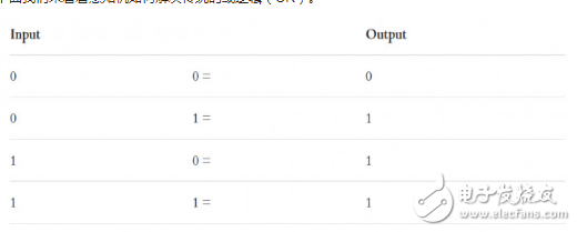
Minsky and Papt's critical perceptrons cannot solve the XOR problem (XOR, requiring 1&1 to return 0):
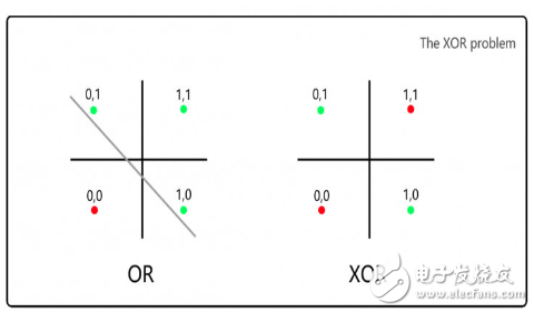
For the OR logic on the left, we can separate the case of 0 and 1 by a line, but for the XOR logic on the right, it cannot be divided by a line.
Artificial neural networks
In 1986, David Everett Rumelhart and Geoffrey Hinton proposed a back propagation algorithm to prove that neural networks can solve complex nonlinear problems. When this theory was put forward, the computer was 1000 times faster than before. Let us see how Rumelhart and others introduced this significant milestone:
We propose a new learning process for neural networks - back propagation. Backpropagation constantly adjusts the connection weights in the network, minimizing the error between the actual output and the desired output. Because of the weight adjustment, we added hidden neurons, which are neither part of the input layer nor the output layer. They extracted the important features of the task and normalized the output. Backpropagating this ability to create effective features distinguishes it from previous algorithms such as the perceptron convergence process.
Nature 323, 533-536 (October 9, 1986)
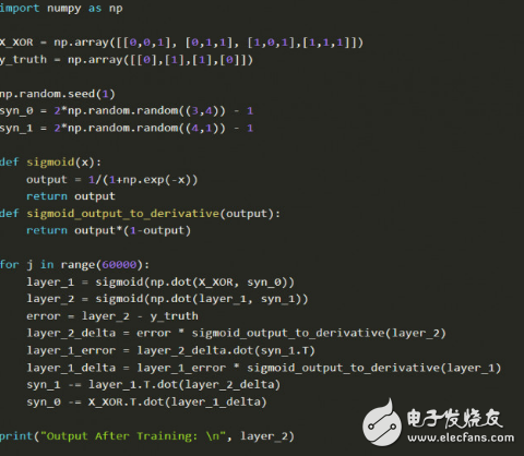
To understand the core of this paper, we implemented the code of DeepMind Andrew Trask, which is not a randomly chosen code. This code was adopted by Andrew Karpathy's in-depth learning course and Siraj Raval in Udacity. More importantly, the idea embodied in this code solves the XOR problem and melts the first winter of AI.
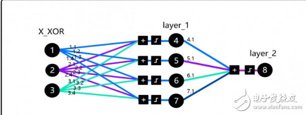
Before we go any further, readers can try this simulator, spend an hour or two to get familiar with the core concepts, then read Trask's blog, and then get familiar with the code. Note that the added parameter in the X_XOR data is a bias neuron, similar to a constant in a linear function.
The combination of backpropagation, matrix multiplication and gradient descent here may circumvent you, and the reader can understand it through the visualization process. Focus on the logic behind it, don't think about it all at once.
In addition, readers can take a look at Andrew Karpathy's back-propagation lesson, take a look at the visualization process, and read Michael Nelsen's book Neural Network and Deep Learning.
Deep neural network
The deep neural network refers to the neural network model of the multi-layer network in addition to the input layer and the output layer. This concept was first proposed by Rina Dechter of the Cognitive Systems Laboratory of the University of California, and can refer to the paper "Learning While". Searching in Constraint-SaTIsfacTIon-Problems, but the concept of deep neural networks only gained mainstream attention in 2012. Soon after IBM IBM Watson won the US Eospardy edge, Google launched cat face recognition.
The core structure of the deep neural network remains unchanged, but it has now been applied to different problems, and the formalization has also been greatly improved. A set of mathematical functions originally applied to simplify noise data is now used in neural networks to improve the generalization of neural networks.
Much of the innovation in deep learning is due to the rapid increase in computing power, which improves the researcher's innovation cycle. Those who originally needed a supercomputer in the mid-eighties to calculate a year's task, today only takes half a second with the GPU. The clock can be completed.
Cost reductions in computing and deeper learning of library resources make it possible for the public to walk into this line. Let's look at an example of a normal deep learning stack, starting with the bottom:
GPU 》 Nvidia Tesla K80. Usually used for image processing, compared to the CPU, they are 50-200 times faster in deep learning tasks.
CUDA GPU's underlying programming language.
CuDNN 》 Nvidia optimizes CUDA library
Tensorflow 》 Google's deep learning framework
TFlearn 》 Tensorflow front-end framework
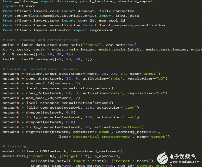
Let's look at an example of a numerical classification (MNIST dataset), which is an entry-level example of the "hello world" of the deep learning community.
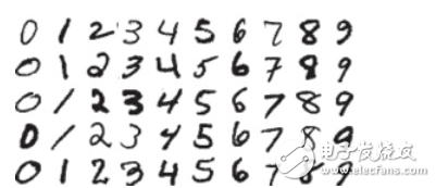
Implemented in TFlearn:
There are many classic articles explaining the MNIST problem, refer to the Tensorflow documentation, the JusTIn Francis article, and the video released by Sentdex.
If you want to know more about TFlearn, you can refer to the blog post by Emil Wallner.
to sum up
As with the TFlearn example above, the main idea of ​​deep learning is still much like the perceptron proposed by Rosenblatt many years ago, but the binary Heaviside step function, the neural network of today, is no longer used. Most use the Relu activation function. At the last level of the convolutional neural network, the loss is set to the multi-class logarithmic loss function categorical_crossentropy, which is a major improvement to the Legendre least squares method, using logistic regression to solve multi-class problems. In addition, the optimization algorithm Adam originated from Derby's gradient descent idea. In addition, Tikhonov's regularization idea is widely applied to the regularization functions of the Dropout layer and the L1 / L2 layer.
KNLE1-63 Residual Current Circuit Breaker With Over Load Protection
KNLE1-63 TWO FUNCTION : MCB AND RCCB FUNCTIONS
leakage breaker is suitable for the leakage protection of the line of AC 50/60Hz, rated voltage single phase 240V, rated current up to 63A. When there is human electricity shock or if the leakage current of the line exceeds the prescribed value, it will automatically cut off the power within 0.1s to protect human safety and prevent the accident due to the current leakage.
leakage breaker can protect against overload and short-circuit. It can be used to protect the line from being overloaded and short-circuited as wellas infrequent changeover of the line in normal situation. It complies with standard of IEC/EN61009-1 and GB16917.1.
KNLE1-63 Residual Current Circuit Breaker,Residual Current Circuit Breaker with Over Load Protection 1p,Residual Current Circuit Breaker with Over Load Protection 2p
Wenzhou Korlen Electric Appliances Co., Ltd. , https://www.korlen-electric.com