Direct code is the most effective way to learn. This tutorial explains the BP backpropagation algorithm with a very simple example implemented in a short Python code.
Of course, the above procedure may be too concise. Below I will briefly break it down into several parts for discussion.
Part 1: A simple neural network
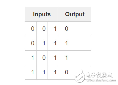
A neural network trained with BP algorithm attempts to predict the output with input.
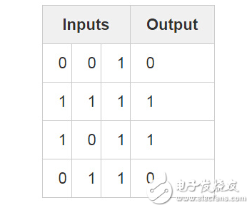
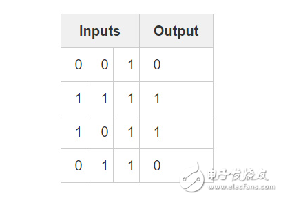
Consider the above scenario: Given three columns of inputs, try to predict the corresponding column of outputs. We can solve this problem by simply measuring the data of the input and output values. In this way, we can see that the leftmost column of input and output values ​​are perfectly matched/fully correlated. Intuitively, the back propagation algorithm uses this method to measure the statistical relationship between data and then obtain the model. Let's go straight to the topic and practice it.
Layer 2 neural network:
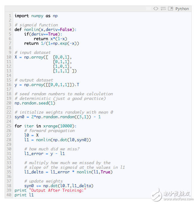
Output After Training:
[[ 0.00966449]
[ 0.00786506]
[ 0.99358898]
[ 0.99211957]]
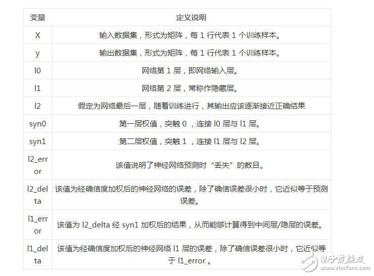
Variable definition
X Enter the data set in the form of a matrix with 1 training sample per row.
y Output dataset in the form of a matrix with 1 training sample per row.
L0 Network layer 1, the network input layer.
L1 Layer 2 of the network, often referred to as the hidden layer.
Syn first layer weight, synapse 0, connect l0 layer and l1 layer.
0
* Multiply by element, so multiplying two equal-length vectors is equivalent to multiplying their equivalent elements, and the result is a vector of equal length.
– The elements are subtracted, so the subtraction of the two equal length vectors is equivalent to the subtraction of the equivalent elements, and the result is a vector of the same length.
X.dot(y) If x and y are vectors, perform dot product operations; if they are matrices, perform matrix multiplication operations; if one of them is a matrix, multiply the vector and matrix.
As seen in the "Results Output after Training", the program executes correctly! Before describing the specific process, I recommend that the reader try to understand and run the code in advance, and have an intuitive feeling about how the algorithm program works. It's best to run the above program in the ipython notebook (or you want to write a script yourself, but I still strongly recommend the notebook). Here are a few key points to help you understand the program:
· Compare the state of the l1 layer at the first iteration and the last iteration.
· Look closely at the "nonlin" function, which gives us a probability value as an output.
· Carefully observe how l1_error changes during the iteration.
· Split the expression in line 36 to analyze, most of the secret weapons are inside.
· Carefully understand the 39th line of code, all operations on the network are preparing for this step.
Let's go through the code line by line.
Suggestion: Open this blog with two screens so you can read the article against the code. I did exactly that when I was writing a blog.
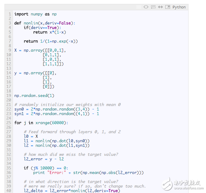
Line 1: Here you import a linear algebra tool library called numpy, which is the only external dependency in the program.
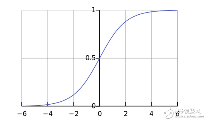
Line 4: Here is our "non-linear" part. Although it can be a lot of functions, here, the nonlinear mapping used is a function called "sigmoid". The Sigmoid function maps any value to a value in the range 0 to 1. Through it, we can convert real numbers into probability values. For the training of neural networks, the Sigmoid function also has several other very nice features.
Line 5: Note that the derivative of the sigmod function is also available through the "nonlin" function body (when the formal parameter deriv is True). One of the excellent features of the Sigmoid function is that its derivative value can be obtained only by its output value. If the output value of Sigmoid is represented by the variable out, its derivative value can be obtained simply by the expression out *(1-out), which is very efficient.
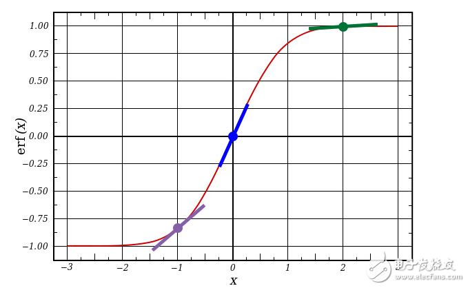
If you are not familiar with the derivative, then you can understand that the derivative is the slope of the sigmod function curve at a given point (as shown in the figure above, the different points on the curve correspond to different slopes). For more information on the derivative, refer to the Khan Institute's Derivative Solving Tutorial.
Line 10: This line of code initializes our input dataset to a matrix in numpy. Each behavior is a "training instance" with one input node for each column. In this way, our neural network has 3 input nodes and 4 training instances.
Line 16: This line of code initializes the output data set. In this case, to save space, I generated the dataset in a horizontal format (1 row and 4 columns). ".T" is the transpose function. After transposition, the y matrix contains 4 rows and 1 column. Consistent with our input, each row is a training instance, and each column (only one column) corresponds to one output node. Therefore, our network has 3 inputs and 1 output.
Line 20: It is a good practice to seed your random number settings. In this way, the weight initialization set you get is still randomly distributed, but each time you start training, the initial set of weights obtained is completely consistent. This makes it easy to see how your strategic changes affect network training.
Line 23: This line of code implements the initialization of the neural network weight matrix. Use "syn0" to refer to "zero synapse" (ie, "input layer - first layer hidden layer" weight matrix). Since our neural network has only 2 layers (input layer and output layer), only one weight matrix is ​​needed to connect them. The weight matrix dimension is (3,1) because the neural network has 3 inputs and 1 output. In other words, the size of the l0 layer is 3, and the size of the l1 layer is 1. Therefore, in order to connect each neuron node of the l0 layer with each neuron node of the l1 layer, a connection matrix of dimension (3, 1) is required. :)
Also, note that the random initialization weight matrix has a mean of 0. There is a lot of knowledge about the initialization of weights. Since we are still only practicing now, it is OK to set the mean to 0 when the weight is initialized.
Another realization is that the so-called "neural network" is actually this weight matrix. Although there are "layers" l0 and l1, they are all based on the instantaneous value of the data set, that is, the input and output states of the layer vary with different input data, and these states do not need to be saved. In the learning training process, only the syn0 weight matrix is ​​stored.
Line 25: The code at the beginning of this line is the code for neural network training. This for loop iteratively executes the training code multiple times, allowing our network to better fit the training set.
Line 28: It can be seen that the first layer l0 of the network is our input data. For this, the following is further elaborated. Remember that X contains 4 training instances (rows)? In this part of the implementation, we will deal with all instances at the same time, this training method is called "batch" training. So, although we have 4 different l0 rows, you can think of them as a single training instance, and there is no difference. (We can load 1000 or even 10,000 instances at once without changing one line of code).
Line 29: This is the forward prediction phase of the neural network. Basically, let the network first "try" to predict the output based on the given input. Next, we will study how the predictions are so effective that some adjustments are made to make the network perform better during each iteration.
(4 x 3) dot (3 x 1) = (4 x 1)
This line of code consists of two steps. First, multiply l0 and syn0 by a matrix. Then, pass the result of the calculation to the sigmoid function. Specifically consider the dimensions of each matrix:
(4 x 3) dot (3 x 1) = (4 x 1)
Matrix multiplication is constrained, for example, the two dimensions of the equation must be consistent. The resulting matrix has the number of rows as the number of rows in the first matrix and the number of columns in the number of columns in the second matrix.
Since 4 training instances were loaded, 4 guess results were obtained, namely a (4 x 1) matrix. Each output corresponds to a guess of the correct result for the given input network. Perhaps this also explains intuitively: why we can "load" any number of training instances. In this case, matrix multiplication still works.
Line 32: Thus, for each input, it is known that l1 has a corresponding "guess" result. Then by subtracting the real result (y) from the guess result (l1), you can compare the effect of the network prediction. L1_error is a vector of positive and negative numbers that reflects how much error the network has.
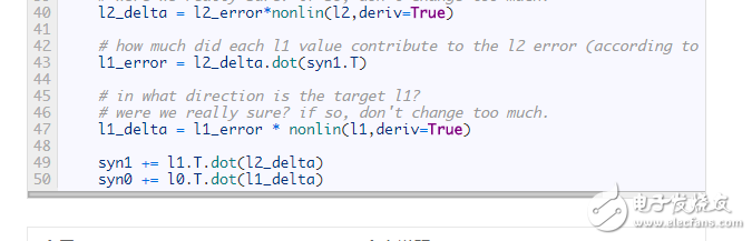
Line 36: Now, we have to run dry goods! Here is the secret weapon! The amount of code in this line is relatively large, so split it into two parts for analysis.
Part I: Derivation
Nonlin(l1,True)
If l1 can be represented as 3 points, as shown in the figure below, the above code can produce three diagonal lines in the figure. Note that if the output value is large at x=2.0 (green dot), and if the output value is small at x=-1.0 (purple point), the slash is very flat. As you can see, the point with the highest slope is at x=0 (blue point). This feature is very important. It can also be found that all derivative values ​​are in the range of 0 to 1.
Overall understanding: error term weighted derivative

Of course, the term "weighted derivative value" is mathematically more rigorously described, but I think this definition accurately captures the intent of the algorithm. L1_error is a (4,1) size matrix, and nonlin(l1,True) returns a (4,1) matrix. What we do is multiply it "elementally" to get a matrix of (4,1) size l1_delta, each of which is the result of multiplication of the elements.
When we multiply the "slope" by the error, we actually reduce the prediction error with high confidence. Looking back at the sigmoid function curve! When the slope is very flat (close to 0), then the network output is either a large value or a small value. This means that the network is very sure whether this is the case or another situation. However, if the judgment result of the network corresponds to (x = 0.5, y = 0.5), it is not so certain. For this "plausible" prediction situation, we make the biggest adjustments to it, and do not deal with the determined situation. Multiply a number close to 0, the corresponding adjustment amount can be ignored.
Line 39: Now, the update network is ready! Let's take a look at the next simple training example.
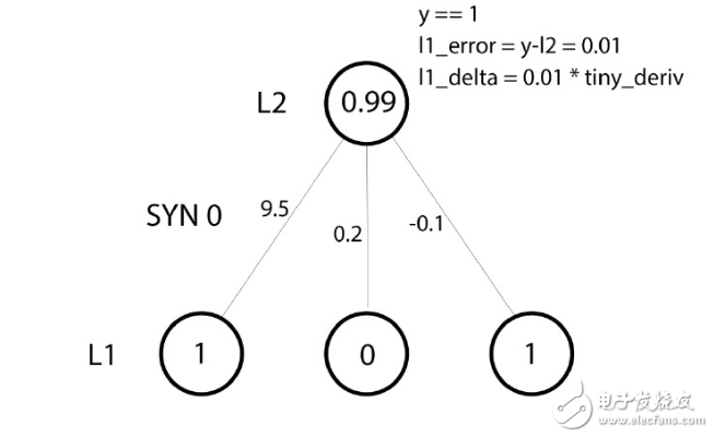
In this training example, we have prepared everything for the weight update. Let us update the leftmost weight (9.5).
Weight update amount = input value * l1_delta
For the leftmost weight, in the above formula, it is 1.0 times the value of l1_delta. As you can imagine, this increment of weights of 9.5 is negligible. Why is there such a small update? It is because we are very convinced of the prediction results, and it is correct to have a good grasp of the prediction results. The error and slope are both small, which means a small update. Considering all the connection weights, the increments of these three weights are very small.
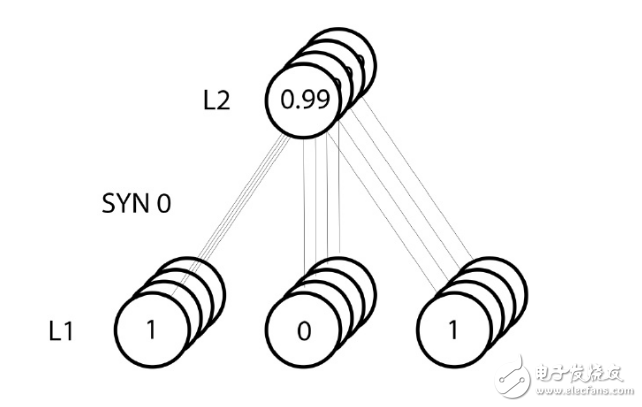
However, since the "batch" training mechanism was adopted, the above update steps were performed on all four training instances, which also looked somewhat similar to the image. So what did line 39 do? In this simple line of code, it completes the following operations: first calculate the weight update amount corresponding to each weight in each training instance, then accumulate all the updates of each weight, and then update These weights. Personally deducing this matrix multiplication operation, you can understand how it does this.
Key conclusions:
Now, we already know how the neural network is updated. Go back and look at the training data and make some deep thoughts. When the input and output are both 1, we increase the connection weight between them; when the input is 1 and the output is 0, we reduce the connection weight
Therefore, in the following four training examples, the weight between the first input node and the output node will continue to increase or remain unchanged, while the other two weights appear to increase or decrease simultaneously during training. (Ignore the intermediate process). This phenomenon allows the network to learn based on the connection between input and output.
Part II: A slightly more complicated issue
Consider the following scenario: Given the first two columns of inputs, try to predict the output column. One key point is that there is no association between the two columns and the output. Each column has a 50% chance of a prediction of 1 and a 50% chance of a prediction of 0.
So what is the current output mode? It seems to be irrelevant to the third column, and its value is always 1. Columns 1 and 2 can be more clearly understood. When 1 column has a value of 1 (but not 1!), the output is 1. Here is the model we are looking for!
The above can be considered a "non-linear" mode because there is no one-to-one relationship between a single input and output. There is a one-to-one relationship between the combination of inputs and the output, which is the combination of column 1 and column 2 here.
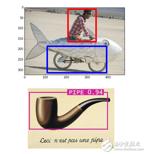
Believe it or not, image recognition is a similar problem. If there are 100 images of the same size of the pipe and the picture of the bicycle, then there is no single pixel position to directly indicate whether a picture is a bicycle or a pipe. From a statistical point of view, these pixels may also be randomly distributed. However, the combination of certain pixels is not random, that is, it is this combination that forms a bicycle or a person.
Our strategy
As can be seen from the above, there is a one-to-one relationship between the product after pixel combination and the output. In order to complete this combination first, we need to add an additional network layer. The first layer combines the inputs and then takes the output of the first layer as input and the final output by the mapping of the second layer. Before giving a concrete implementation, let's look at this table.
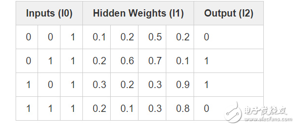
After the weights are randomly initialized, we get the hidden value of layer 1. Did you notice anything? The second column (the second hidden layer node) has a certain correlation with the output! Although not perfect, it is also remarkable. Whether you believe it or not, finding this correlation accounts for a large percentage of neural network training. (It can even be assumed that this is the only way to train neural networks.) What the subsequent training has to do is to increase this association further. The syn1 weight matrix maps the combined output of the hidden layer to the final result, and while updating syn1, the syn0 weight matrix needs to be updated to better produce these combinations from the input data.
Note: Model more combinations of relationships by adding more middle tiers. This strategy is well-known as "deep learning" because it is modeled by continuously adding deeper layers of the network.
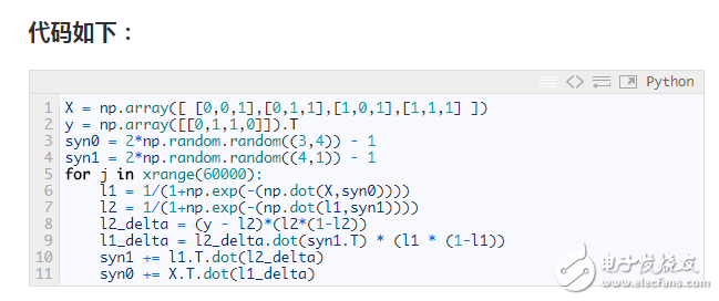
Everything looks so familiar! This is just a stack of two previous implementations, the output of the first layer (l1) being the input to the second layer. The only new thing that appears is the line 43 code.
Line 43: The corresponding error of the l1 layer is constructed by "confidence weighting" the error of the l2 layer. In order to do this, simply pass the error between l2 and l1 to pass the error. This approach can also be called “contribution weighting error†because we are learning how much the output value of each node of the l1 layer contributes to the l2 layer node error. Next, the syn0 weight matrix is ​​updated using the same steps in the previous two-layer neural network implementation.
Part III: Summary
If you want to understand the neural network carefully, give you some advice: try to reconstruct this network with memory. I know it sounds crazy, but it does help. If you want to be able to create neural networks of arbitrary structures based on new academic articles, or to read sample programs of different network structures, I think this training will be a killer. This can be helpful even when you are using some open source frameworks such as Torch, Caffe or Theano.
Aluminum Alloy LED lamps,Low Power LED lamps,LED wall washer
Kindwin Technology (H.K.) Limited , https://www.ktlleds.com