In process control, the PID controller controlled by the ratio of deviation (P), integral (I) and differential (D) is the most widely used automatic controller. It has the advantages of simple principle, easy implementation, wide application range, independent control parameters, simple selection of parameters, etc.; and theoretically, it can be proved that the typical object of process control--"first-order lag + pure lag" and The control object of "second-order lag + pure lag", PID controller is an optimal control. The PID regulation law is an effective method for dynamic quality correction of continuous systems. Its parameter setting method is simple and the structure changes flexibly (PI, PD, ...).

PID is a closed-loop control algorithm

Therefore, to implement the PID algorithm, you must have closed-loop control on the hardware, that is, you must have feedback. For example, to control the speed of a motor, you must have a sensor that measures the speed and feed the result back to the control route. The speed control is also taken as an example below.
PID is proportional (P), integral (I), differential (D) control algorithm
But it is not necessary to have these three algorithms at the same time, it can also be PD, PI, or even only P algorithm control. One of my simplest ideas for closed-loop control was P control, which feeds back the current results and subtracts them from the target. If it is positive, it will decelerate. If it is negative, it will accelerate. Now know that this is just the simplest closed loop control algorithm.
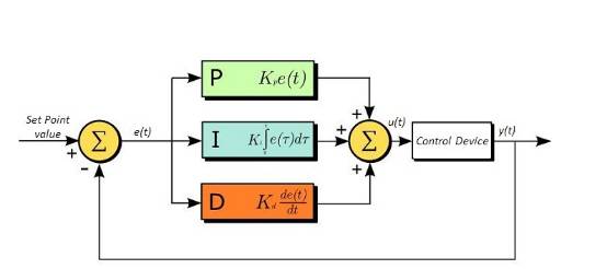
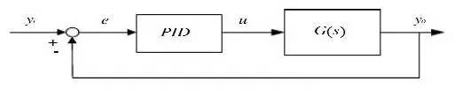
PID controller structure
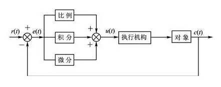
PID control system principle block diagram
The proportional, integral and differential operations of the deviation signal are transformed to form a control law. “Using deviations to correct deviationsâ€.
Analog PID controller
Analog PID controller structure
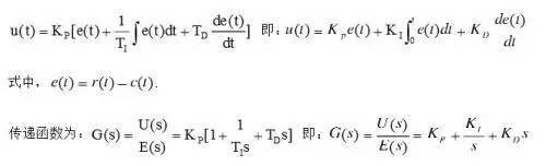
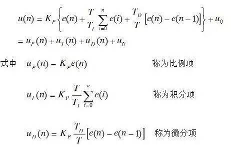
The input and output relationship of the PID controller is:

Proportional (P), integral (I), and differential (D) control algorithms have their own effects
Proportion, the basic (current) deviation e(t) of the reaction system, the coefficient is large, which can speed up the adjustment and reduce the error, but the excessive ratio makes the stability of the system decrease, and even the system is unstable;
Integral, the cumulative deviation of the reaction system, so that the system eliminates the steady-state error and improves the no-difference. Because of the error, the integral adjustment is performed until there is no error;
Differential, reflecting the rate of change of the system deviation signal e(t)-e(t-1), is predictive, can predict the trend of deviation change, and produces advanced control effect. It has been differentially adjusted before the deviation has not formed. Eliminated, thus improving the dynamic performance of the system. However, the differential has an amplification effect on the noise interference, and the enhanced differentiation is detrimental to the system's anti-interference. Both integration and differentiation cannot work alone and must be coordinated with proportional control.
Controller P, I, D item selection
The following summarizes the control characteristics of various commonly used control laws:
(1) Proportional control law P: The P control law can quickly overcome the influence of disturbance. Its effect on the output value is fast, but it can not be stabilized at an ideal value. The bad result is more effective. Overcoming the effects of disturbances, but there is a surplus. It is suitable for occasions where the control channel has less hysteresis, the load changes little, the control requirements are not high, and the controlled parameters are allowed to have a margin within a certain range. Such as: the water pump room cooling and hot water level control under the Jinyu Public Works Department; the oil level control of the oil pump house.
(2) Proportional integral control law (PI): Proportional integral control law is the most widely used control law in engineering. The integral can eliminate the residual on the basis of the ratio. It is suitable for occasions where the control channel has less hysteresis, the load does not change much, and the controlled parameter does not allow the residual. Such as: heavy oil flow control system of F1401 to F1419 gun in heavy oil reversing room of main line kiln head; oil supply pipe flow control system of oil pump house; temperature regulation system of each area of ​​annealing kiln.
(3) Proportional differential control law (PD): The differential has a leading role. For the control channel with capacity lag, the differential participation control is introduced. When the differential term is set properly, it has a significant effect on improving the dynamic performance index of the system. . Therefore, in the case where the time constant or capacity hysteresis of the control channel is large, in order to improve the stability of the system, the dynamic deviation can be reduced, and the proportional differential control law can be selected. Such as: heating type temperature control, composition control. It should be noted that for those areas with pure hysteresis, the differential term is powerless, and in systems where the signal is noisy or periodically vibrating, differential control is not appropriate. Such as: the control of the glass level of the big kiln.
(4), example integral differential control law (PID): PID control law is an ideal control law, which introduces the integral on the basis of the proportion, can eliminate the residual, then add the differential action, and can improve the stability of the system. Sex. It is suitable for occasions where the control channel time constant or capacity lag is large and the control requirements are high. Such as temperature control, composition control, etc.
In view of the role of the D law, we must also understand the concept of time lag, which includes capacity lag and pure lag. The capacity lag usually includes: measurement lag and transmission lag. Measuring hysteresis is a kind of hysteresis that the detecting component needs to establish a balance when detecting, such as thermocouple, thermal resistance, pressure, etc., which is slow to respond. The transmission lag is a kind of control lag generated by sensors, transmitters, actuators and other equipment. Pure hysteresis is relative and measurement lag. In industry, most of the pure lag is caused by material transfer. For example, the kiln glass level requires a long period of time during the action of the feeder to the nuclear level meter.
In short, the selection of the control law should be selected according to the process characteristics and process requirements. It is by no means that the PID control law has better control performance under any circumstances, and it is unwise to adopt it regardless of the occasion. If you do this, it will only add complexity to other work and bring difficulties to parameter tuning. When the PID controller is used, the other control schemes need to be considered. Such as cascade control, feedforward control, large hysteresis control, etc.
The setting of three parameters of Kp, Ti and Td is a key issue of the PID control algorithm. Generally speaking, only the approximate values ​​of them can be set during programming, and the optimal value is determined by repeated debugging while the system is running. Therefore, the debugging phase program must be able to modify and memorize these three parameters at any time.
Digital PID controller
(1) Discretization of simulated PID control law
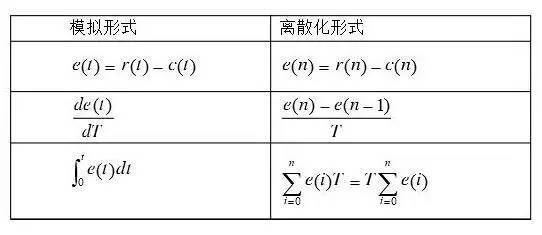
(2) Difference equation of digital PID controller
Self-tuning of parameters
In some applications, such as the general instrument industry, the working object of the system is uncertain. Different objects have to adopt different parameter values. If the parameters cannot be set for the user, the concept of parameter self-tuning is introduced. The essence is to find a set of parameters for the new work object through N measurements when first used, and remember it as the basis for future work. There are three specific tuning methods: critical proportionality method, attenuation curve method, and empirical method.
1. Critical proportionality method (Ziegler-Nichols)
1.1 Under the pure proportional action, gradually increase the gain to generate the secondary vibration, and obtain the PID controller parameters according to the critical gain and critical period parameters. The steps are as follows:
(1) Connect the pure proportional controller to the closed-loop control system (set the controller parameter integral time constant Ti = ∞, the actual differential time constant Td =0).
(2) The controller proportional gain K is set to the minimum, and the step disturbance (generally changing the given value of the controller) is added to observe the step response curve of the adjusted amount.
(3) Change the proportional gain K from small to large until the closed loop system oscillates.
(4) When the system exhibits constant amplitude oscillation, the gain at this time is the critical gain (Ku), and the oscillation period (time between peaks) is the critical period (Tu).
(5) The PID controller parameters are derived from Table 1.
Table 1
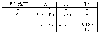
1.2 The following points should be noted in the timing of the critical proportional method:
(1) When using this method to obtain the equal-amplitude oscillation curve, the control system should be operated in the linear region, and the control valve should not be opened or closed. Otherwise, the continuous oscillation curve obtained may be the "limit cycle". The linear system conceptually says that the system is already in divergence.
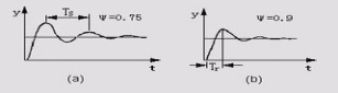
(2) Due to the different characteristics of the controlled object, the controller parameters obtained according to the above table may not always obtain satisfactory results. For the object without self-balancing characteristics, the controller parameter obtained by the critical proportional method is too large to make the system response attenuation rate (ψ>0.75). For high-order isometric objects with self-balancing characteristics, the system response attenuation rate is mostly small when using this method to adjust the controller parameters (ψ<0.75). To this end, the controller parameters obtained above should be corrected online during the actual operation of the specific system.
(3) The critical proportionality method is applicable to process control systems with small critical amplitude and long oscillation period, but some systems do not allow stable boundary tests, such as boiler drum water level control systems, from safety considerations. There are also some single-capacity objects with large time constants. The system is always stable when using pure proportional control. For these systems, the critical scaling method cannot be used for parameter tuning.
(4) It is only applicable to higher-order objects of second order or higher, or objects of first-order plus pure lag. Otherwise, in the case of pure proportional control, the system will not exhibit equal-amplitude oscillation.
1.3 If the static magnification KP=Δy/△u of the controlled object is obtained, the gain product KpKu can be regarded as the maximum open loop gain of the system. The scope of application of the Ziegler-Nichols closed-loop test setting method is generally considered to be:
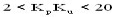
(1) When KpKu > 20, more complicated control algorithms should be used for better adjustment.
(2) When KpKu < 2, some control strategies that compensate for the transmission delay should be used.
(3) When 1.5
(4) When KpKu < 1.5, the PI controller can still be used in the case where the control accuracy is not high. In this case, the differential action has little meaning.
2. Attenuation curve method
The difference between the attenuation curve method and the critical proportional method is that the closed-loop set value perturbation test uses attenuated oscillation (usually 4:1 or 10:1), and then uses the experimental data of the damped oscillation to determine the controller according to the empirical formula. parameter. The tuning steps are as follows:
(1) Under the pure proportional controller, the proportional gain K is set to a small value and the system is put into operation.
(2) After the system is stable, make a set value step disturbance and observe the response of the system. If the system response decays too fast, reduce the proportional gain K; otherwise, increase the proportional gain K. Until the system exhibits a 4:1 damped oscillation process as shown in Fig. 1(a), note the proportional gain Ks and the oscillation period Ts at this time.
figure 1
(3) Using the Ks and Ts values, calculate the parameter setting values ​​of the controller according to the empirical formula given in Table 2.
Table 2

(4) The 10:1 attenuation curve method is similar, but is calculated by Tr.
There are a few points to note when using the attenuation curve method:
(1) Adding a given disturbance can not be too large, it should be determined according to the requirements of production operations, generally around 5%, and there are exceptions.
(2) It is necessary to add a given disturbance when the process parameters are stable, otherwise the correct tuning parameters will not be obtained.
(3) For systems with fast response, such as flow rate, pipeline pressure and small-capacity liquid level adjustment, it is difficult to obtain a strict 4:1 attenuation curve. Generally, the parameter is fluctuated twice to achieve stability, which is approximately It is considered that the 4:1 attenuation process is reached.
(4) When putting into operation, first put K at a small value, reduce Ti to the setting value, gradually increase Td to the setting value, and then pull K to the setting value (if K=setting value is very Quickly put Td to the setting, the output of the controller will change drastically).
3. Experience setting method
3.1 Method One A:
(1) Determine the proportional gain
Make the PID purely proportional. The input is set to 60%~70% of the maximum allowable value of the system. The proportional gain is gradually increased from 0 to the oscillation of the system. Conversely, the proportional gain from this time gradually decreases until the system oscillation disappears. The proportional gain at this time is recorded, and the proportional gain P of the PID is set to be 60% to 70% of the current value.
(2) Determine the integral time constant
After the proportional gain P is determined, the initial value of a large integral time constant Ti is set, and then Ti is gradually decreased until the system oscillates, and then, in turn, Ti is gradually increased until the system oscillation disappears. Record Ti at this time, and set the integration time constant Ti of the PID to 150% to 180% of the current value.
(3) Determine the integral time constant Td
The integral time constant Td is generally not required to be set and is 0. To set, as in the method of determining P and Ti, take 30% of the oscillation.
(4) The system carries the joint adjustment, and then fine-tunes the PID parameters until the requirements are met.
3.2 Method One B:
(1) PI adjustment
(a) Under the action of pure proportionality, gradually reduce the proportionality from a large value to the beginning of the periodic oscillation (the measured value oscillates regularly with a given value), and in the case of periodic oscillation, This proportion is gradually widened until the system is fully stabilized.
(b) Next, the integration time is gradually shortened to generate oscillation. At this time, the integration time is too short, and the integration time should be slightly extended until the oscillation stops.
(2) PID adjustment
(a) Seeking the vibration point under pure proportional action.
(b) Increase the differential time to stop the oscillation, then adjust the proportional slightly smaller, so that the oscillation is generated again, increase the differential time, stop the oscillation, and operate back and forth until the differential time is increased, but it cannot be made. The oscillation stops and the optimum value of the differential time is obtained. At this time, the proportionality is adjusted slightly larger until the oscillation stops.
(c) Adjust the integration time to the same value as the derivative time. If oscillation occurs again, increase the integration time until the oscillation stops.
3.3 Method 2:
Another method is to take a certain value of Ti from the range of the table. If it needs to be differentiated, take Td=(1/3~1/4)Ti, then try to make δ, and it can reach faster. Claim. Practice has proved that by appropriately combining the values ​​of δ and Ti within a certain range, a curve with the same attenuation ratio can be obtained, that is, the decrease of δ can be compensated by increasing Ti, without substantially affecting the quality of the adjustment process. Therefore, in this case, it is also possible to determine Ti, Td and then determine the order of δ. And maybe faster. If the curve is still not ideal, Ti and Td can be adjusted appropriately.
3.4 Method 3:
(1) In the actual debugging, you can also set an empirical value first, and then modify according to the adjustment effect.
Flow system: P (%) 40--100, I (minutes) 0.1--1
Pressure system: P (%) 30--70, I (minutes) 0.4--3
Liquid level system: P (%) 20--80, I (minute) 1-5
Temperature system: P (%) 20--60, I (minutes) 3--10, D (minutes) 0.5--3
(2) The following stipulations:
The step disturbance is closed to the closed loop, and the parameter is set to see the curve; the first is to cast the proportional and then the integral, and finally the differential is added;
Two waves of ideal curve, the amplitude is attenuated by 4 to 1; the ratio is too strong to oscillate, and the integral is too strong;
The motion difference is too large and differential, the frequency is too fast and the differential is reduced; the deviation from the fixed value is slow, and the integral action is strengthened.
4. Parameter tuning of complex adjustment system
The cascade adjustment system is taken as an example to illustrate the parameter tuning method of the complex adjustment system. Since there are two sets of parameters, the main and the sub-parameters in the cascade adjustment system, there is a mutual connection and influence between each channel and the circuit. Changing any of the parameters of the primary and secondary loops has an effect on the overall system. Especially when the time constants of the primary and secondary objects are not much different, the dynamic connection is close, and the work of setting parameters is particularly difficult.
Before setting the parameters, it is necessary to clarify the design purpose of the cascade regulation system. If the quality of the main parameters is mainly guaranteed, and the requirements for the sub-parameters are not high, the setting work is relatively easy; if the main and auxiliary parameters are required to be high, the setting work is more complicated. The following describes the two-step parameter tuning method of “first deputy and second masterâ€.
The first step: in the case of stable conditions, the main circuit is closed, the main controller proportionality is placed at 100%, the integration time is placed at the maximum, and the derivative time is placed at zero. The secondary loop is calibrated with a 4:1 attenuation curve, and the proportional gain K2s and the oscillation period T2s of the secondary loop are obtained.
The second step is to regard the secondary circuit as a link of the main circuit, and use the 4:1 attenuation curve method to set the main circuit to obtain the main controllers K1s and T1s.
Calculate the primary and secondary loop parameters of the cascade regulation system according to the empirical formula of Table 2 according to K1s, K2s, T1s, and T2s. Put the secondary loop parameters first, then put the main loop parameters. If a satisfactory transition process is obtained, the tuning is completed. Otherwise, appropriate adjustments can be made.
If the time constants of the primary and secondary objects are not much different, according to the 4:1 attenuation curve method, there may be a “resonance†hazard. In this case, the secondary loop proportionality or integration time can be appropriately reduced to reduce the secondary loop oscillation period. purpose. For the same reason, increase the main circuit proportionality or integration time, in order to increase the main circuit oscillation period, so that the ratio of the main and sub-circuit oscillation periods is increased to avoid "resonance". The result of this will reduce the quality of the adjustment.
If the characteristics of the primary and secondary objects are too close, it means that the determined scheme is not proper, and the tuning can not be completely relied on to improve the quality of the adjustment.
Practical application experience:
First, the digital PID control algorithm is used to adjust the speed of the DC motor. The solution is to use the photoelectric switch to obtain the pulse signal generated by the rotation of the motor. The single chip (MSP430G2553) calculates the rotation speed of the motor by measuring the frequency of the pulse signal (the specific measurement frequency algorithm is Using direct measurement method, how many pulses are measured at 1s, the measurement error of the measurement can be 0.5 rpm plus or minus), and the measured rotation speed is compared with the given rotation speed to generate an error signal to generate a control signal. The control signal is adjusted by PWM. The duty cycle is also controlled by adjusting the output analog voltage (equivalent to a 1-bit DA. If a 10-bit DA is used for analog adjustment? Will the effect be much better?), this experimental control capability has a certain range. It can only be controlled between 30 rev / sec and 150 rev / sec. When the given value (the speed given in the program) is higher than 150, the actual speed can only be maintained at 150 rpm, which is the maximum of this system. Control ability, when the set value is lower than 30 revolutions, the DC motor shaft does not actually rotate, but because the error value is too large, the speed will rapidly become high, It will stop rotating, and thus the cycle, can not achieve the control effect.
According to the actual measurement, the steady-state accuracy of the rotational speed is within plus or minus 3 revolutions, and the control time is 4 to 5 seconds. Experiments only go to this level, thinking and analysis only stay at this depth.
The second is to use the digital PID control algorithm to adjust the position of the DC geared motor. The solution is to measure the position and angle of the motor rotation by using a precision potentiometer rotating coaxially with the motor. The angle and position obtained by the measurement are compared with the given position. The error signal, then the position error signal is converted into a PWM signal through a certain relationship (this relationship is purely based on imaginary and experimental phenomena), and the PWM signal as the control signal is the first to generate an analog voltage U, U for the DC geared motor. To control the torque of the DC geared motor (not clear), the torque generates acceleration, the acceleration produces the speed, the speed changes position, and the output is the position signal. Therefore, the system should be modeled and analyzed for the DC geared motor, and the DC geared motor should be simulated. Approximate system transfer function, and then according to this function, the parameters of the PID can be set.
The two experiences are not particularly clear how the PID parameters are set. There is no clear theoretical guidance and experimental steps, and the results are not organized and analyzed in time, resulting in the depth and extent of the experiment can not achieve the desired results.
Cob Lights ,Cob Led Strip,Cob Led Light,Cob Strip Light
Guangzhou Cheng Wen Photoelectric Technology Co., Ltd. , https://www.cwledwall.com